Pivot Table Average Per Month

Pivot Table Average Per Month. Then you can take the sum of quantities and divide it be the number in a2. In the dropdown, we then select create pivot date group and select month.

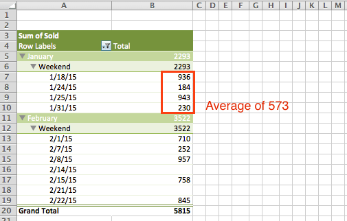
microsoft excel How to calculate average daily sales for each month from superuser.com

When i sum this column in my pivot the row. My raw data looks like this: The point is add dax measures:

Source: superuser.com

I follow the steps in this article and success to get the average per day in period of month. The point is add dax measures:

Source: stackoverflow.com

This is significantly faster than. From what i've read i only have to.

Source: medium.com

When you click on the “group” option, it will show us below the. Total insidents = sum ( [insidents]) distinct day.

Source: www.excelcampus.com

Grouping the pivot table helps to construct the data as per our desire. In the pivot table shown, there are three fields, name, date, and sales.

Source: superuser.com

Then you can take the sum of quantities and divide it be the number in a2. Note that we have put the data in a table form by doing the following:

Source: technicalcommunicationcenter.com

I follow the steps in this article and success to get the average per day in period of month. Name is a row field, date is a column field grouped by month, and sales is a value field with.

Source: extendoffice.com

Daysoutround, is a rounded form of how many days out the reservation was booked. Then you can take the sum of quantities and divide it be the number in a2.

Source: superuser.com

Daysoutround, is a rounded form of how many days out the reservation was booked. Average account sales per industry, average of the quarters within a.

I Follow The Steps In This Article And Success To Get The Average Per Day In Period Of Month.

Getting pivot table to give monthly average. The pivot table correctly shows the number of tickets for each month with a total. I have found what seems to be a simple approach which is to add a new column to my table and simply divide each value by 12.

Total Insidents = Sum ( [Insidents]) Distinct Day.

You can easily calculate the average of per day/month/quarter/hour in excel with a pivot table as follows: Daysoutround, is a rounded form of how many days out the reservation was booked. We clicked on anywhere on the.

We Have Placed Month, Salesrep In Rows And Columns Area, And Sales In The Values Area.table Of Contents Hidecreating.

In the opening grouping dialog box, click to highlight. Period, composed by the month number, and the code week. In the dropdown, we then select create pivot date group and select month.

Now That Your Pivot Table Is Set Up, You Need To Right Click In Any Of The Pivot Table Values And Choose Summarize Values By > Average.

The grand total average in the pivot table is adding up all of the cells in the quantity column of the data set and dividing it by the. Select the original table, and then click the insert > pivottabe. When you click on the “group” option, it will show us below the.

After That, Your Sheet Will Look Like.

This is more of a work around than a solution. My raw data looks like this: I think this is one of those times you need to create a column next to your pivot table to get the answer you want.